

During a crisis, people tend to criticize the ones that were supposed to prepare for it. Whatever has been done, it’s not good enough: There was too little preparation, the response was too late. But before the crisis existed the same people often were criticized too: Their proposed measures were too expensive and too restrictive. The difference is that we prepare for a risk, but we have to deal with a problem.
CISO Says... Lies, damn lies! [statistics]
July 2, 2019 at 11:50
How viable is traditional IT risk analysis[1]?
Part I – Probability
IT security essentially reduces information-related risk to an acceptable ratio of risk to cost. For this reason, the process begins with an extensive risk assessment – a tried and tested process that can be improved. I am inspired by the work of Douglas Hubbard[2] on this topic. Here’s why.

Traditional risk analysis starts by creating a list of things that could go wrong. We estimate the maximum impact as well as probability and we multiply these figures to “calculate” the risk.
In some cases, this works reasonably well. The (financial) risk of a laptop being stolen from a parked car can be estimated like this. When a company owns a few thousand laptops it will happen several times per year. After a few years the number becomes predictable. The value of a laptop is harder to estimate. During presentations, when I ask the value of a laptop I’m holding up, the response of the audience is usually in the range of the list price of the laptop. After I tell them it holds the only copy of a research project someone has been working on for six weeks, the estimates inevitably rise. The estimates might increase further once we know that the laptop has shareholder information or a customer database saved on its hard drive.
Not all laptops will contain this kind of valuable information. However, these variables are often not adequately addressed in traditional IT risk management. The standard risk calculation is as follows: estimation laptop is stolen is 2% (per year), estimation laptops containing valuable information is 50%, probability of risk is 2% x 50%=1% (per year).
Even for such a simple risk calculation, the analysis is elusively complex. Risks with a very high impact and a low probability are even more elusive. What if your company is put on some blacklist and your cloud-based system, including all your data, becomes unavailable because the provider is not allowed to do business with you anymore? Not a very likely scenario, I admit, but what if this provider was hacked or goes bankrupt? This scenario is perhaps more probably. Worst case you lose all your data, but again this is not very likely. In traditional risk analyses the risk will be calculated using maximum impact:
risk = (almost zero) x (ridiculous amount of money) = nonsense.
Reality is not black and white. The impact of an unwanted event is not zero or maximum damage. Fire in the datacentre is usually very local, because of a failing power supply. A datacentre burning down to the ground is not very common. The damage in any incident will most likely be in the range of tens of thousands of euro’s, the maximum damage will be a number of millions. The fact that damage is probably a lot lower in most cases is completely ignored with this method.
One may argue, for absolute values the traditional methods are not ideal, but at least it’s one strategy to use when prioritizing risk.
In traditional risk analysis risks are categorized in levels of impact (Negligible, minor, moderate, …) and levels of likelihood (improbable, seldom, occasional, …). A matrix is created where all the identified risks are plotted. Usually it is color-coded to categorize high impact and high probability (red), low impact and low probability (green) and everything in between (gradients). It’s often called a heatmap.
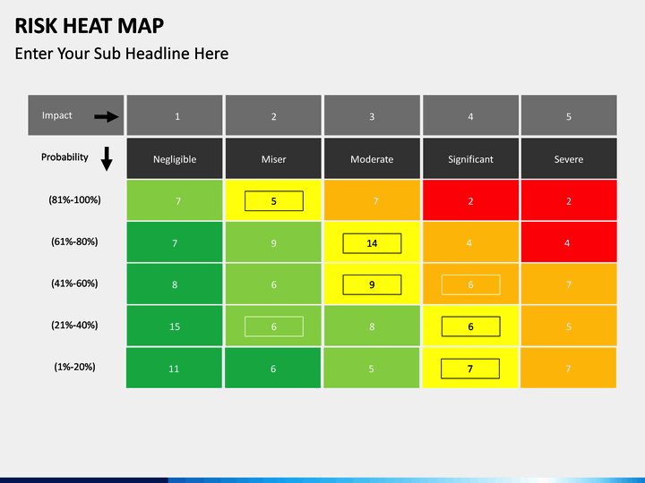
Hubbard gives a few examples in his book[3]. For this example, the category “seldom” is defined as >1%-25% and category “catastrophic” as >10 Million like in the heatmap example above. Let’s assume we identified two risks:
-
risk A: likelihood is 2%, impact in 10 Million
- risk B: likelihood is 20%, impact is 100 Million
When we calculate the risk as likelihood x impact, risk B is 100 times risk A. They would however be plotted in the same cell of the matrix. In the same way you could end up with risks which are very similar but end up in different cells.
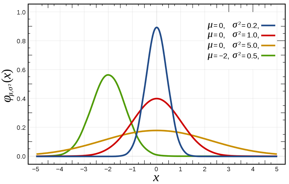
A way to address the fact that there is variance in the impact of any event is to assume that the probability of any amount of damage will follow a normal distribution[4]. A normal distribution is shown in the diagram below. The mean value will have the highest probability, very low and very high values will have a low probability, meaning that the bandwidth will vary. In the diagram below the blue line the mean value for blue, red and yellow lines is zero. The probability we are between -0.5 and 0.5 is much higher with the blue line than with the yellow line.
Applied to the stolen laptop example the risk can now be defined as:
Risk = (2% chance per year a laptop is stolen) x (90% probability the impact is between 1000 and 25000 euro)
A giant data leak may occur resulting in millions of damages when a single laptop is stolen, the probability however is very low (less than 5%, probably lower).
Note we now define the risk as a change or probability of damage instead of an absolute amount of money. In my opinion, this models the real world, where we can predict the course of the impact of events happening, but we cannot predict the impact of individual events. People who play the lottery will “win” about half of the money they pay for their tickets, but the chance of someone winning the jackpot is miniscule.
Part II of this mini-series within the ‘CISO Says’ blogs will address how a curve can be properly identified.
Sources:
[1] https://en.wikipedia.org/wiki/Lies,_damned_lies,_and_statistics
[2] https://en.wikipedia.org/wiki/Douglas_W._Hubbard
[3] How to Measure Anything in Cybersecurity Risk, Douglas W. Hubbard, ISBN 9781119085294, (p90)
[4] https://en.wikipedia.org/wiki/Central_limit_theorem