

IT security essentially reduces information related risk to an acceptable ratio of risk to cost. For this reason, the process begins with an extensive risk assessment – a tried and tested process that can be improved. I am inspired by the work of Douglas Hubbard on this topic. Here’s why - part III.
CISO Says... Lies! - PART II
August 5, 2019 at 12:55
IT security essentially reduces information related risk to an acceptable ratio of risk to cost. For this reason, the process begins with an extensive risk assessment – a tried and tested process that can be improved. I am inspired by the work of Douglas W. Hubbard[1] on this topic. Here’s why ‘Part II’.
In part one of the blog, I explained the shortcomings of traditional IT risk assessment where we calculate risk as likelihood x maximum expected damage. I introduced an alternative where the expected damage is not a fixed amount, but follows a curve. We will now address how the curve (Probability Density Function) can be properly identified and created.
We estimate the probability that an event will occur (likelihood) in the traditional way and then combine this with the curve to calculate an expected loss. I will also go into greater depth on how to adjust the parameters of the curve to locate the best possible fit for its function.
Probability density function
The probability of damage incurred will follow a normal distribution. A nice visualisation of this is the Galton Board [2]. Hubbard argues that the best model for security related events is normal distribution on a logarithmic scale (lognormal). It represents a common situation where risk cannot result in damage lower than zero and risk can result, yet unlikely, in very high damage (p41) [3]. Information security risk are not necessarily tangible, but they are undoubtedly part of reality.
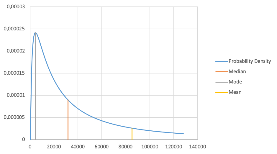
Figure 1: Lognormal probability density
Two given points on this curve are sufficient to calculate the complete curve. To ensure that it is simplified as possible, we choose the 90% confidence interval. This means we can estimate a lower and upper bound of the expected damage in 9 out of 10 events, for instance: in 9 out of 10 times the damage of a stolen laptop is between €2000 and €500k (Figure 1). To estimate the upper and lower bound Hubbard encourages us to use all data available. Even small samples are valuable. When we have only 5 samples there is already a more than 90% probability the median [4] value is between the highest and lowest sampled value (p32). The median in this example is about €31.600; if there were at least five laptops stolen last year, then at least one of them is expected to have caused a lower damage and at least one of them is expected to have caused a higher damage. If this is not the case, we should probably adjust the upper and lower bounds.
The probability that an event will happen
The probability an event will happen (likelihood), is measured in one percentage point over the course of one year. Therefore, a 10% likelihood means we expect the event to happen once every 10 years.
When historical data is available, we are obliged to use it – luckily, we are not limited to our own data sets. It is possible to access data from similar situations or similar companies. When an event happened twice in a span of three years within a sample group of seven companies, we know the probability of the event occurring is about 2/(3x7 )=9.5%. Note this figure is fact based, not an estimation!
Expected inherent loss
Combining the curve and likelihood we can calculate the expected inherent loss per year for this risk. Using Hubbard’s formula [5] there is an expected inherent loss of €12,300 per year in our example. Calculating the expected loss before and after application of a security control is a way to measure the yield of the implemented control.
Choosing the probability density functions parameters
Since the expected inherent loss is based on the upper & lower bound and the probability of loss, there are many ways to choose these parameters resulting in the same expected inherent loss.
As an example, consider the following options where we vary the lower bound and the probability of loss in order to keep the Expected Inherent Loss more or less constant.

These parameters result in the following probability density distributions (Figure 2).
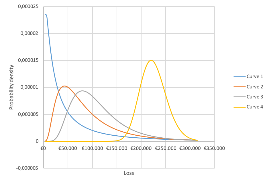
Figure 2: Varying the lower bound and probability of loss
Each curve models a different situation. The blue line models a situation with many laptops imposing a relatively low damage when stolen, while the yellow curve models a situation with many laptops imposing a relatively high damage when stolen. The expected loss is similar because the effect is compensated by the probability the event will happen (see table). The difference, however, is quite big (9,5% vs 4,85%) and the yellow line is probably too extreme in our example.
The blue line however, is quite extreme too. This is due to the upper and lower bound being so far apart. Hubbard warns for unrealistic outcomes if the spread between the upper bound and the lower bound is too large (p42).
Suppose we have five or more samples (laptops stolen) and at least one of the cases the damage was higher than €70,711 and at least one case resulting in damage lower than that. These cases would fit the orange curve which has a lower bound of €10.000 instead of €2000. We probably underestimated the lower bound.
If we adjust the lower bound, but want to keep the expected loss unchanged, we have to adjust the probability an event will happen from 9,5% to 8,5%. This seems a reasonable deviation from the 9.5% we calculated. If we keep this to 9,5% the expected loss will rise to €13.623.
Why calculation matters
The expected inherent loss is defined as what the business is expected to lose in a year because of the identified risk. A company will generally have budget for these losses as a part of the normal operating cash flows, so minimizing expected loss can free up capital for other investments. In essence, our calculations contribute to the overall budget allocation of our clients.
Of course, a company will have multiple risks and they may not be all as straight forward as in the examples given. With my next blog installation, we will look into dealing with more complex risks and a way to calculate the total amount of risks.
Sources:
[1] https://en.wikipedia.org/wiki/Douglas_W._Hubbard
[2] https://www.youtube.com/watch?v=EvHiee7gs9Y
[3] The page numbers in brackets refer to How to Measure Anything in Cybersecurity Risk, Douglas W. Hubbard, ISBN 9781119085294.
[4] The median value is by definition the value any sample has a probability of 50% being lower and 50% being higher than the median. The chance 5 consecutive random samples are all higher is 50%x50%x50%x50%x50%=3,125%. All samples lower is another 3.125%, leaving 100%-2x3.125%=93,75% chance the median is between the samples. On a logarithmic scale, this is applied to ln(value).
[5] Taken from his example Excel sheet: https://www.howtomeasureanything.com/cybersecurity/wp-content/uploads/sites/3/2019/06/OneforOne-Substitution-Model-2019c-HTMA-Cybersecurity-Version.xlsx